- Victor Yuan/
- Posts/
- "Can you check gene x for me?" quickly reading 1 gene at a time from single cell data/
"Can you check gene x for me?" quickly reading 1 gene at a time from single cell data
“Can you check gene x for me?” is a common question I get when working with other scientists on gene expression projects. This is an easy task after setting up a gene expression web apps with shiny. Though, one pain point for specficially single cell data is that app start up and general data queries become quite slow if using standard analytical single cell packages like Seurat and others. For example, a 500 000 cell dataset can take up to 40 seconds to load into memory. Increasingly, I need to check a gene in not just one, but multiple single cell datasets. In my current system of loading entire single cell datasets into memory, this is terribly inefficient for what is essentially a simple task.
How can we optimize these queries so that instead of taking minutes, it only takes seconds?
Well, rather than loading the entire data into memory, can we load only the relevant portion, i.e. a gene of interest?
Single cell formats
If we distill this task into a more general one - loading a single row / slice from rectangular data, then there are many options that exist. However, for single cell RNAseq data there are other considerations:
data for single cell is often the order of 20,000 - 40,000 genes, often arranged in rows, and 100 000 - 1 million cells in the columns. It does not often travel in “tidy” formats (e.g. with columns gene, cell, value).
single cell count matrix usually travels as sparse matrix due to high drop-out rate. Coercion to dense is resource-heavy so need to do this thoughtfully and only when necessary.
For this post I explore how to utilize the HDF5 format to speed up reading 1 gene at a time into R, in order to address memory and speed issues when working with large and multple single cell datasets.
Options for using HDF5 with single cell data
Actually, there is already a great memory-efficient solution out there called ShinyCell, which utilizes the HDF5 format, and produces a clean, fast, memory-efficient shiny-based app. It looks like ShinyCell has it’s own approach to writing single cell count data to h5 format.
I think this is interesting because there are already some existing h5 formats already designed for single cell data, like python’s .h5ad and h5Seurat. And in contrast to these ones, Shinycell writes a dense count matrix, rather than the other formats mentioned which keep the format of the data as sparse. This makes sense though as the goal of these other formats is to provide entry to existing tools that work with sparse data.
So I will compare ShinyCell’s rather manual h5 strategy to some other options. The other option included here is HDF5Array + delayedArray, which are some Bioconductor options specifically for Bioconductor-specific data structures, like scRNAseq.
Key packages for this post
For HDF5, there are a couple of general purpose options in R: hdf5r, rhdf5. Then there is the bioconductor package HDF5Array which uses hdf5r in backend to work with bioconductor data structures specifically.
Other packages
HDF5Array hdf5 read write dense/sparse matrices
hdf5r hdf5 r implementation
scRNAseq to access example scRNAseq dataset
tidyverse glue gt fs general purpose
tictoc bench timing
library(HDF5Array)
library(hdf5r)
library(scRNAseq)
library(tidyverse)
library(tictoc)
library(withr)
library(bench)
library(gt)
library(glue)
library(fs)
sce <- ZilionisLungData()## see ?scRNAseq and browseVignettes('scRNAseq') for documentation## loading from cache## see ?scRNAseq and browseVignettes('scRNAseq') for documentation## loading from cachecounts <- sce@assays@data$counts[,]Saving dgc matrix manually with hdf5r
This is ShinyCell’s approach, which is to write the sparse count matrix of a Seurat / SingleCellExperiment object to a dense representation on disk. Because converting the sparse matrix to dense would implode most computers, shinycell’s approach is to do this in chunks / loops.
I modify the code to make it easier to follow, and I litter the function with tictoc::tic and toc to monitor the overall and each step takes.
Alternatively, we could write sparse representation to disk, which would be faster to write (less data), but then we would need to convert to dense on the read-in endpoints. I don’t do that here, because the goal is to speed up read-in, not write-out. Though it may be trivially fast to coerce a 1 x 1million vector? Am not sure.
file_h5 <- fs::path('counts.h5')
if (file.exists(file_h5)) file.remove(file_h5)
## [1] TRUEwrite_dgc_to_h5 <- function(dgc, file, chunk_size = 500) {
# open h5 connection and groups
h5 <- H5File$new(file, mode = "w")
on.exit(h5$close_all())
h5_grp <- h5$create_group("grp")
h5_grp_data <- h5_grp$create_dataset(
"data",
dtype = h5types$H5T_NATIVE_FLOAT,
space = H5S$new("simple", dims = dim(dgc), maxdims = dim(dgc)),
chunk_dims = c(1, ncol(dgc))
)
tic('total')
for (i in 1:floor((nrow(dgc) - 8)/chunk_size)) {
index_start <- ((i - 1) * chunk_size) + 1
index_end <- i * chunk_size
tic(glue::glue('loop {i}, rows {index_start}:{index_end}'))
h5_grp_data[index_start:index_end, ] <- dgc[index_start:index_end,] |>
as.matrix()
toc(log = TRUE)
}
# final group
index_start <- i*chunk_size + 1
index_end <- nrow(dgc)
tic(glue::glue('final loop, rows {index_start}:{index_end}'))
h5_grp_data[index_start:index_end, ] <- as.matrix(dgc[index_start:index_end, ])
toc(log = TRUE)
# add rownames and colnames
h5_grp[['rownames']] <- rownames(dgc)
h5_grp[['colnames']] <- colnames(dgc)
toc()
}
write_dgc_to_h5(counts, file_h5, chunk_size = 1000)## loop 1, rows 1:1000: 7.81 sec elapsed
## loop 2, rows 1001:2000: 7.06 sec elapsed
## loop 3, rows 2001:3000: 7.02 sec elapsed
## loop 4, rows 3001:4000: 6.97 sec elapsed
## loop 5, rows 4001:5000: 8.73 sec elapsed
## loop 6, rows 5001:6000: 6.5 sec elapsed
## loop 7, rows 6001:7000: 7.19 sec elapsed
## loop 8, rows 7001:8000: 6.92 sec elapsed
## loop 9, rows 8001:9000: 6.84 sec elapsed
## loop 10, rows 9001:10000: 6.58 sec elapsed
## loop 11, rows 10001:11000: 6.41 sec elapsed
## loop 12, rows 11001:12000: 6.78 sec elapsed
## loop 13, rows 12001:13000: 6.39 sec elapsed
## loop 14, rows 13001:14000: 7.28 sec elapsed
## loop 15, rows 14001:15000: 6.33 sec elapsed
## loop 16, rows 15001:16000: 6.67 sec elapsed
## loop 17, rows 16001:17000: 6.83 sec elapsed
## loop 18, rows 17001:18000: 7.31 sec elapsed
## loop 19, rows 18001:19000: 6.39 sec elapsed
## loop 20, rows 19001:20000: 6.67 sec elapsed
## loop 21, rows 20001:21000: 6.86 sec elapsed
## loop 22, rows 21001:22000: 7.36 sec elapsed
## loop 23, rows 22001:23000: 6.38 sec elapsed
## loop 24, rows 23001:24000: 6.75 sec elapsed
## loop 25, rows 24001:25000: 6.78 sec elapsed
## loop 26, rows 25001:26000: 7.09 sec elapsed
## loop 27, rows 26001:27000: 6.14 sec elapsed
## loop 28, rows 27001:28000: 12.68 sec elapsed
## loop 29, rows 28001:29000: 7.09 sec elapsed
## loop 30, rows 29001:30000: 7.56 sec elapsed
## loop 31, rows 30001:31000: 6.66 sec elapsed
## loop 32, rows 31001:32000: 10 sec elapsed
## loop 33, rows 32001:33000: 10.42 sec elapsed
## loop 34, rows 33001:34000: 8.59 sec elapsed
## loop 35, rows 34001:35000: 7.61 sec elapsed
## loop 36, rows 35001:36000: 8.1 sec elapsed
## loop 37, rows 36001:37000: 6.54 sec elapsed
## loop 38, rows 37001:38000: 8.5 sec elapsed
## loop 39, rows 38001:39000: 6.71 sec elapsed
## loop 40, rows 39001:40000: 7.42 sec elapsed
## loop 41, rows 40001:41000: 12.31 sec elapsed
## final loop, rows 41001:41861: 8.39 sec elapsed
## total: 315.11 sec elapsedRead 1 gene at a time
Now to define a function that opens the h5 file, reads the particular slice of data we want, and then close the h5 file. It is important to ensure the file gets closed, otherwise it can get corrupt. This is a bit of a drawback for this approach, but I have yet to encounter a problem so far.
read_gene <- function(gene, file_h5) {
  #tic('whole thing')
  stopifnot(file.exists(file_h5))
  # open connections
  #tic('open')
  h5 <- H5File$new(
    file_h5,
    mode = "r")

  #on.exit(h5$close_all())

  h5_data <- h5[['grp']][['data']]
  h5_rownames <- h5[['grp']][['rownames']]
  h5_colnames <- h5[['grp']][['colnames']]

  #toc()
  #tic('read gene')
  ind <- str_which(h5_rownames[], gene)
  #ind <- 18871
  #print(ind)
  gene <- h5_data[ind,]
  #toc()

  #tic('set name')
  gene <- setNames(gene, nm = h5_colnames[])
  #toc()

  #tic('close')
  h5$close_all()
  #toc()
  #toc()
  return(gene)
}


gene <- read_gene('AC006486.2', file_h5)
HDF5array
Bioconductor has the HDF5array R package that supports writing / loading dense and sparse matrices from .h5 files.
Let’s see how this compares to the manual implementation.
First write to disk using HDF5Array::writeHDF5Array
file_h5array <- fs::path('HDF5array.h5')
if (file.exists(file_h5array)) file.remove(file_h5array)
## [1] TRUEtic();HDF5Array::writeHDF5Array(
DelayedArray(counts),
file_h5array, as.sparse = FALSE, name = 'full', with.dimnames = TRUE);toc()## <41861 x 173954> HDF5Matrix object of type "double":
## bcIIOD bcHTNA bcDLAV ... bcELDH bcFGGM
## 5S_rRNA 0 0 0 . 0 0
## 5_8S_rRNA 0 0 0 . 0 0
## 7SK 0 0 0 . 0 0
## A1BG 0 0 0 . 0 0
## A1BG-AS1 0 0 0 . 0 0
## ... . . . . . .
## snoZ278 0 0 0 . 0 0
## snoZ40 0 0 0 . 0 0
## snoZ6 0 0 0 . 0 0
## snosnR66 0 0 0 . 0 0
## uc_338 0 0 0 . 0 0## 466.64 sec elapsedh5ls(file_h5array) # see content of h5## group name otype dclass dim
## 0 / .full_dimnames H5I_GROUP
## 1 /.full_dimnames 1 H5I_DATASET STRING 41861
## 2 /.full_dimnames 2 H5I_DATASET STRING 173954
## 3 / full H5I_DATASET FLOAT 41861 x 173954Point to the hf5 file
hf5 <- HDF5Array(file_h5array,  name = 'full', as.sparse = TRUE)
hf5['AC006486.2',] |>  head()
## bcIIOD bcHTNA bcDLAV bcHNVA bcALZN bcEIYJ
## 0 0 0 0 0 0Explore the class
showtree(hf5)## 41861x173954 double, sparse: HDF5Matrix object
## └─ 41861x173954 double, sparse: [seed] HDF5ArraySeed objectshowtree(hf5[2,])## double: [seed] numeric objectclass(hf5)## [1] "HDF5Matrix"
## attr(,"package")
## [1] "HDF5Array"is(hf5, 'DelayedMatrix')## [1] TRUECompare HDF5array vs diy implementation
Now we have written the count matrices to disk in hdf5 format in two ways: manually, and through HDF5Array.
Let’s see if there are differences in performance in reading 1 gene at a time.
Memory and time
bench_read <- bench::mark(
  HDF5Array = hf5['AC006486.2',],
  `h5 - manual` = read_gene('AC006486.2', file_h5),
  `in-memory slice` = counts['AC006486.2',]
)

summary(bench_read) |>
  mutate(expression = as.character(expression)) |>
select(-memory, -result, -time, -gc) |> gt()| expression | min | median | itr/sec | mem_alloc | gc/sec | n_itr | n_gc | total_time |
|---|---|---|---|---|---|---|---|---|
| HDF5Array | 1.7s | 1.7s | 0.5875962 | 10.11MB | 0 | 1 | 0 | 1.7s |
| h5 - manual | 774.7ms | 774.7ms | 1.2908001 | 4.97MB | 0 | 1 | 0 | 774.7ms |
| in-memory slice | 154.5ms | 210.9ms | 5.0724987 | 3.93MB | 0 | 3 | 0 | 591.4ms |
bench_read |> autoplot(type = 'jitter')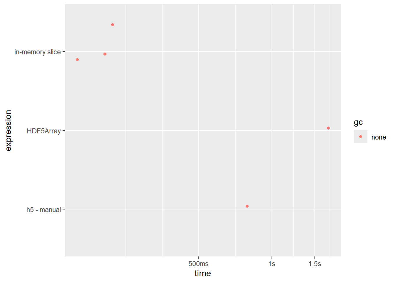
HDF5array is ~2x slower than ShinyCell’s manual method
ShinyCell approach is almost as fast as holding in memory, without of course the cost is occupying a large amount of memory at any given time.
on-disk space
data.frame(file = c(file_h5, file_h5array)) |>
  mutate(file_size = fs::file_size(file))
## file file_size
## 1 counts.h5 153.28M
## 2 HDF5array.h5 221.88MSingleCellExperiment
In reading HD5Array docs, I learned that you can back a SingleCellExperiment object with a HDF5-backed matrix. This is actually incredibly useful, because now we can use any packages for SingleCellExperiment (like tidySingleCellExperiment).
sce_h5 <- SingleCellExperiment(assays = list(counts = hf5))Size of SingleCellExperiment object backed by HDF5
object.size(sce_h5) |> print(units = 'auto')## 9.1 MbSize of dgc counts matrix held in memory
object.size(counts) |> print(units = 'auto')## 624.4 MbSpeed:
bench::mark(sce_h5['AC006486.2',]) |> select(-c(result:gc)) |> gt()| expression | min | median | itr/sec | mem_alloc | gc/sec | n_itr | n_gc | total_time |
|---|---|---|---|---|---|---|---|---|
| [, sce_h5, AC006486.2, | 81.4ms | 83.5ms | 11.77477 | 7.49MB | 0 | 6 | 0 | 510ms |
Conclusion
HDF5format is great for memory efficient loading of single cell data, particularly for single gene queries which take less than 1 second on a 200,000 cell dataset.- The manual
shinyCellh5 method is almost twice as fast asHDF5Array(~1 second vs 0.5 second) - but
SingleCellExperimentcan carry hdf5-backed count matrices withHDF5Array, making it more useful as it opens usage to other single cell tools - The majority of time reading from
HDF5is actually closing the connection of the file.